ecoforge R package

What is ecoforge?
The purpose of ecoforge is to simulate natural processes in space for subsequent analysis. This package enables you to:
Create new spatial environmental layers (predictors)
Adjust a spatial suitability layer based on this environmental layers, and distribute species’ individuals weighted by this layer
Implement different field-based sampling designs
Conversion of the sampled data into formats ready for statistical analysis (abundance and presence/absence data)
With an extra example to check the collinearity between variables.
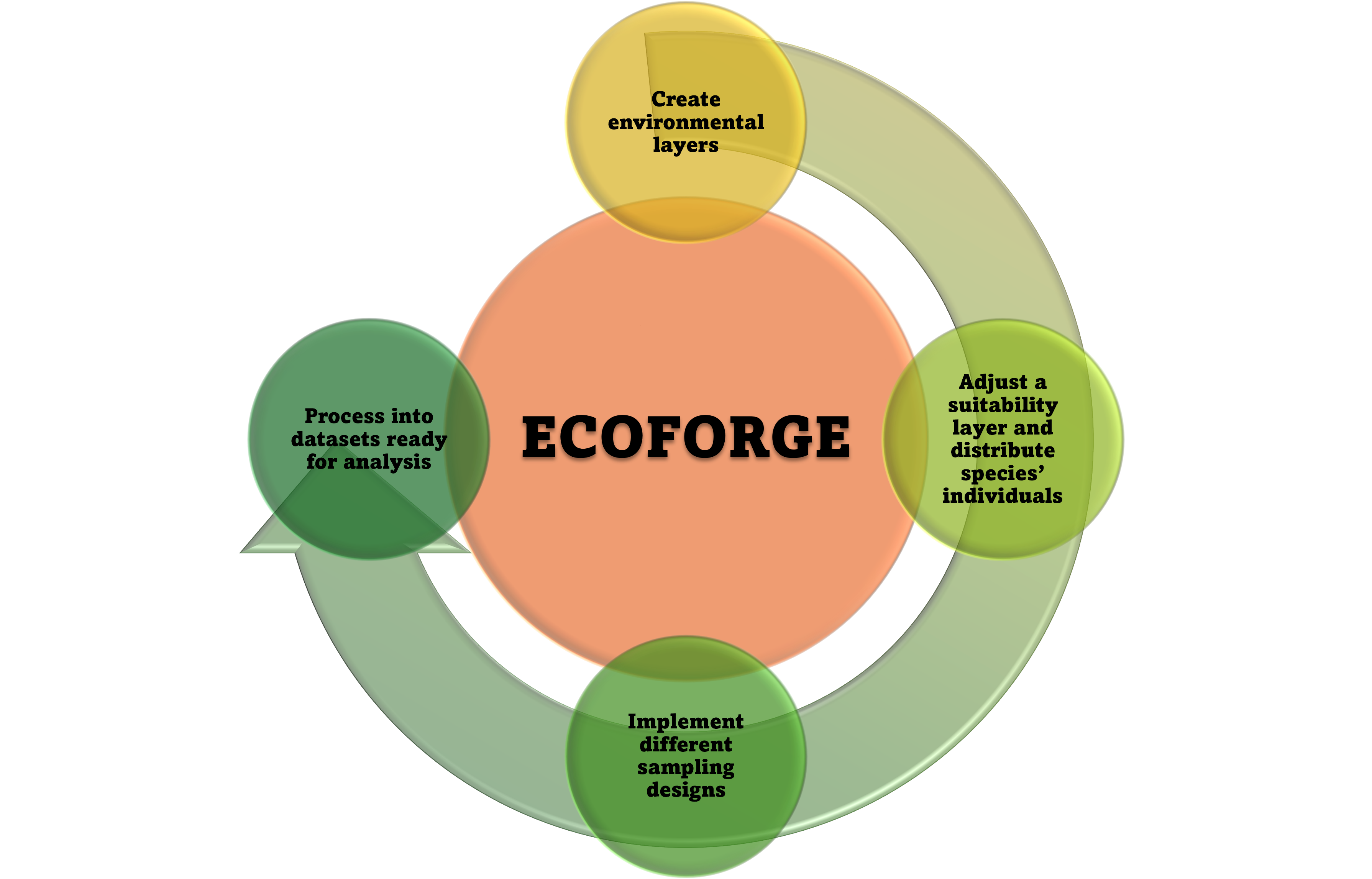
It allows researchers to:
Simulate spatial layers of environmental variables with varying degrees of spatial autocorrelation (climate, vegetation, land use, etc.).
Generate spatial layers of environmental suitability for virtual species, as well as distribute individuals as spatial points across their surface.
Apply different sampling strategies (using point counts or transects, and employing uniform or random sampling) to the simulated individuals.
Convert the simulated data into presence/absence or count formats ready for use in various spatial ecology models (e.g., habitat selection studies, species distribution models, etc.).
This website provides all the information and details about the functions included in the package, as well as some examples of complete simulation vignettes.
When should I use ecoforge?
ecoforge is particularly useful when controlled and reproducible scenarios are needed. For example:
- Testing the performance of spatial models under known conditions
- Evaluating the effect of different possible artefacts, related with sampling design or ecological aspects, on model accuracy
- Teaching and demonstrating concepts in ecological modelling
Installation
# install.packages("devtools")
devtools::install_github("NatureProtectionDFF/Ecoforge-R-package")

library(ecoforge)
ls("package:ecoforge")
Functions Workflow and Reference
ecoforge functions are organized following the logical steps of a virtual ecology workflow. Functions are grouped according to the procedure being carried out: (A) generating the spatial patterns of environmental variables, (B) adjusting that information into a species’ suitability/expected abundance layer, and distributing its individuals within this layer, (C) implementing of different field-based sampling designs to collect data, and (D) conversion of the sampled data into formats ready for statistical analysis (Figure 2). Although the functions are typically chained in this order, each one returns a standard R object (a data frame, a SpatRaster, or a spatstat ‘ppp’ object) and can equally be combined with other packages, or used independently of the rest of the pipeline.
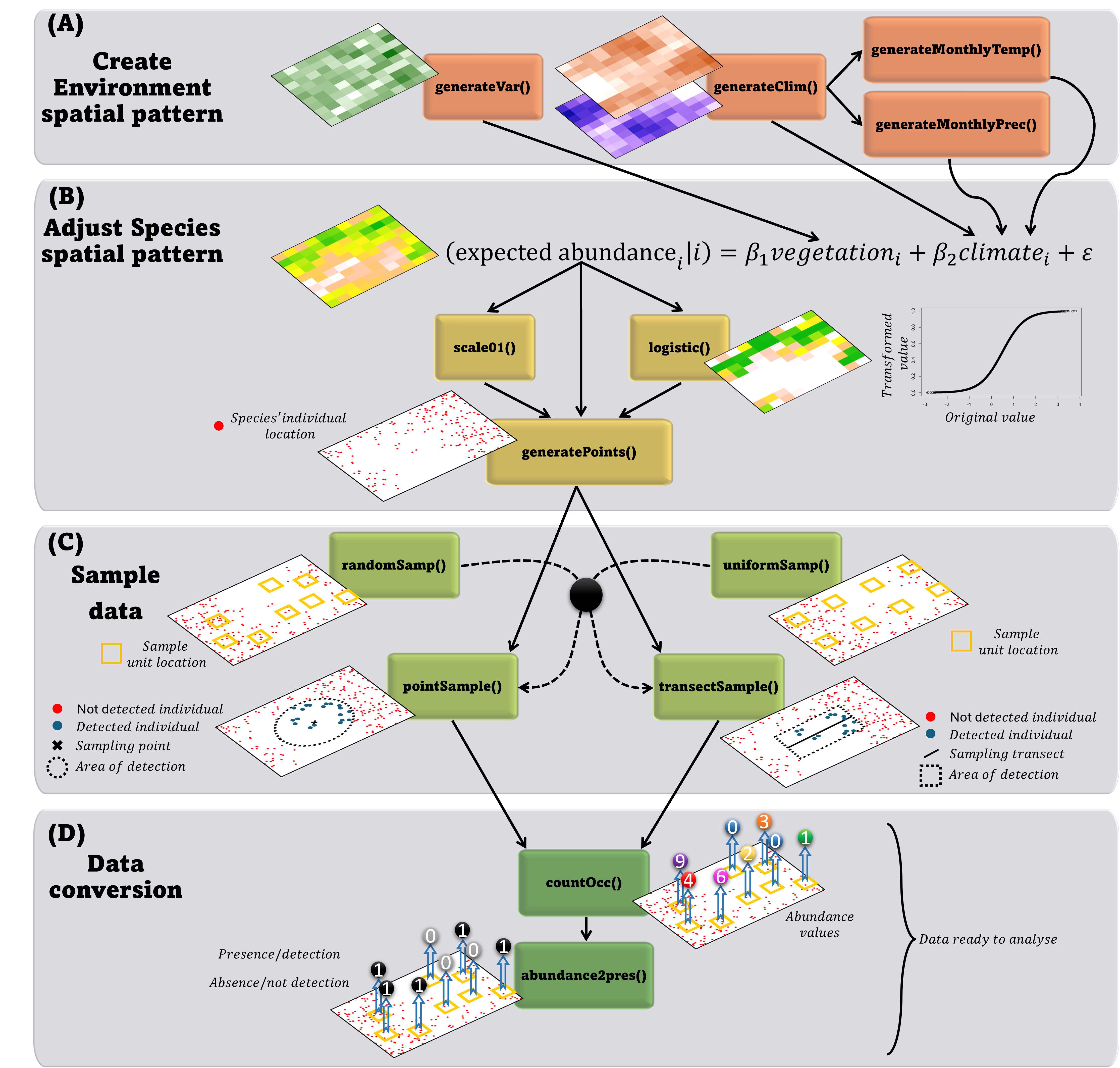
Create environment spatial pattern
Functions to generate modulated spatially autocorrelated environmental variables using Gaussian simulations with a Spherical model based on gstat package.
| Function | Description |
|---|---|
generateVar() |
Generates a single variable (e.g. vegetation, terrain) with modulated spatial autocorrelation |
generateClim() |
Generates a full climate dataset including temperature and precipitation with modulated spatial autocorrelation |
generateMonthlyTemp() |
Derives monthly minimum, average and maximum temperature from annual data, based on ‘generateClim()’ output |
generateMonthlyPrec() |
Derives monthly precipitation from annual data with seasonal pattern, based on ‘generateClim()’ output |
Adjust species’ spatial pattern
Utility functions to modulate the species’ suitability/expected abundance pattern or rescale values. Also use this spatial pattern to distribute species’ individuals or occurrences within this layer extension, employing an inhomogeneous Poisson point process based on spatstat package.
| Function | Description |
|---|---|
scale01() |
Linearly rescales any variable to the [0, 1] range |
logistic() |
Applies a logistic transformation to control distibution of data frequency |
generatePoints() |
Distributes individuals as points across the landscape according to habitat suitability |
Sample data
Functions to first define survey locations and and then simulate field sampling procedures, returning detection distances for each individual inside the detection area of the sampling unit.
| Function | Description |
|---|---|
uniformSamp() |
Places survey sites on a regular systematic grid |
randomSamp() |
Places survey sites at random positions within a grid |
pointSample() |
Simulates point count surveys within a detection radius |
transectSample() |
Simulates line transect surveys within a detection range |
Data conversion
Functions to convert raw sampling output (distances for each individual inside the detection area) into formats ready for the models to be applied (counts, presence/absence, detections/not detections).
| Function | Description |
|---|---|
countOcc() |
Counts of detected individuals per survey site |
abundance2pres() |
Converts abundance counts to presence/absence considering imperfect detection |
Available vignettes
Citation
For now, there is only one article available that uses some of its features as a reference. So if you use ecoForge in your research, please cite this work:
- Ferrer-Ferrando, D., Tarroso, P., Luis Tellería, J., Acevedo, P. and Fernández-López, J. (2025), Disentangling the effect of the spatial scale and species spatial pattern on the abundance–suitability relationship. Ecography, 2025: e07766. https://doi.org/10.1111/ecog.07766
We will soon have a software note focused on this package available as a citation reference.